How to Create Star Ratings for Numbers Using the REPT Function in MS Excel

 Star ratings are a simple and effective way to visually represent numerical values in Microsoft Excel. Whether you are working with customer feedback, employee performance, product scores, survey results, or project evaluations, converting numbers into star ratings can make your spreadsheet easier to understand at a glance.

The good news is that you don't need complicated VBA code, add-ins, or advanced Excel features to create a basic star-rating system. The REPT function can do the job with a simple formula.

In this guide, you'll learn how to create a dynamic star rating in Excel using the REPT function and how to make the result more useful with a few additional techniques.

What Is the REPT Function in Excel?

The REPT function repeats a specified text a particular number of times.

The syntax is:

=REPT(text, number_times)

For example:

=REPT("*",5)

returns:

*****

Here, Excel repeats the * character five times.

This makes REPT particularly useful for creating simple visual indicators such as:

• Star ratings
• Progress bars
• Performance indicators
• Repeated symbols
• Text-based charts
• Visual scorecards

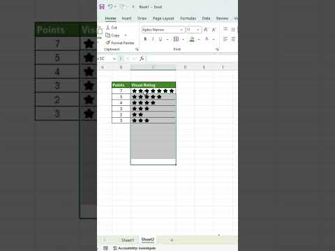
For a star-rating system, we can simply tell Excel to repeat the star character according to the numerical rating.

Creating a Basic Star Rating

Suppose you have a list of products and their ratings.

Product	Rating
Product A	5
Product B	4
Product C	3
Product D	2
Product E	1

Let's assume the rating is in cell B2.

In another column, enter:

=REPT("★",B2)

If B2 contains 5, Excel will display:

★★★★★

If B2 contains 4, it will display:

★★★★

And if B2 contains 2, the result will be:

★★

The formula automatically changes the number of stars according to the value in the rating cell.

Using the Traditional Asterisk Symbol

If you don't want to use the Unicode star character, you can also use an asterisk.

For example:

=REPT("*",B2)

A rating of 5 would produce:

*****

However, the filled star character ★ generally provides a more recognizable rating display.

You can copy and paste this character directly into your formula:

=REPT("★",B2)

Creating a Five-Star Rating System

A common rating system uses a maximum score of five.

For example:

Rating	Star Rating
1	★
2	★★
3	★★★
4	★★★★
5	★★★★★

The formula remains very simple:

=REPT("★",B2)

If the rating changes from 3 to 5, the displayed stars automatically change from three to five.

This is especially useful when your ratings are stored as numerical data and you want to create a more visually appealing report.

Displaying Both Rating and Stars

You may want to display the actual number alongside the visual rating.

For example:

5 ★★★★★

You can combine the rating and REPT function using the & operator:

=B2&" "&REPT("★",B2)

If B2 contains 4, the result will be:

4 ★★★★

This can be useful when readers need both the numerical score and the visual representation.

Creating a Fixed Five-Star Scale

There is another useful approach: displaying both filled and empty stars.

For example:

• 5 → ★★★★★
• 4 → ★★★★☆
• 3 → ★★★☆☆
• 2 → ★★☆☆☆
• 1 → ★☆☆☆☆

This makes it immediately clear that the maximum rating is five.

Assuming the rating is in B2, use:

=REPT("★",B2)&REPT("☆",5-B2)

The first REPT creates the filled stars, while the second creates the remaining empty stars.

For example, if B2 contains 3:

★★★☆☆

If B2 contains 4:

★★★★☆

And if B2 contains 5:

★★★★★

This is one of the easiest ways to create a professional-looking five-star rating system using only an Excel formula.

Adding a Rating Label

You can also display a text label along with the stars.

For example:

=REPT("★",B2)&" "&B2&"/5"

A rating of 4 would display:

★★★★ 4/5

Alternatively, you could place the number first:

=B2&"/5 "&REPT("★",B2)

Result:

4/5 ★★★★

This can be useful for dashboards, reports, product reviews, and survey summaries.

Handling Blank Cells

If your rating column contains blank cells, you may want the star-rating column to remain blank instead of displaying an error or unwanted result.

You can use the IF function:

=IF(B2="","",REPT("★",B2))

This tells Excel:

• If B2 is blank, display nothing.
• Otherwise, repeat the star according to the rating.

For a fixed five-star system:

=IF(B2="","",REPT("★",B2)&REPT("☆",5-B2))

This keeps your worksheet clean when some ratings have not yet been entered.

Making the Star Rating More Attractive

Once your formula is working, you can improve its appearance using Excel formatting.

1. Increase the Font Size

Select the star-rating cells and increase the font size. Larger stars are easier to read in dashboards and reports.

2. Change the Font

Try fonts that display Unicode star characters clearly.

3. Center the Stars

Use Home → Alignment → Center to position the ratings neatly within the cells.

4. Adjust Column Width

Make sure the column is wide enough to display all five stars without cutting them off.

5. Use Conditional Formatting

You can also use conditional formatting to visually distinguish different rating levels.

For example, you could create different formatting rules for ratings of:

• 1–2
• 3
• 4–5

This can make a larger report easier to scan.

Creating Star Ratings for Decimal Numbers

What if your ratings aren't whole numbers?

Suppose your rating is:

4.5

A formula such as:

=REPT("★",B2)

is not ideal for decimal values because REPT needs a meaningful repeat count.

If your rating system should use whole stars, you can round the value.

For example:

=REPT("★",ROUND(B2,0))

A value of 4.4 would be rounded to 4, while 4.6 would be rounded to 5.

You can also use ROUNDUP or ROUNDDOWN depending on how you want decimal ratings to be represented.

Preventing Ratings Above Five

If your data isn't guaranteed to contain values between 1 and 5, it's a good idea to control the input.

You can use Data Validation to restrict ratings to a range of 1 through 5.

Go to:

Data → Data Validation

Then configure the rule to allow a whole number between 1 and 5.

This prevents someone from accidentally entering values such as 7 or -1.

You can also make the formula more robust by using MIN and MAX:

=REPT("★",MAX(0,MIN(5,B2)))

This limits the displayed rating to the 0–5 range.

Using REPT to Create Simple Visualizations

The usefulness of REPT isn't limited to star ratings.

Because it repeats characters based on a numerical value, you can use it to create simple text-based visualizations.

For example:

=REPT("■",B2)

could create a basic bar:

■■■■■

You could also use symbols such as:

●●●●●
█████
★★★★★

This makes REPT a surprisingly useful function for creating lightweight visual indicators without inserting charts.

Where Can You Use Star Ratings in Excel?

Star ratings can be useful in many types of spreadsheets.

Customer Feedback

Convert customer scores into visual ratings so managers can quickly identify highly rated and poorly rated services.

Product Evaluation

Display product ratings in an inventory or product-performance report.

Employee Performance

Use ratings to represent scores for different performance categories.

Survey Analysis

Turn survey scores into visual indicators that are easier to interpret.

Project Evaluation

Use stars to represent project performance, priority, quality, or completion levels.

Dashboards

Star ratings can add a visual element to KPI dashboards without taking up much space.

A Few Useful REPT Formulas

Here are some formulas you can save for future Excel projects:

Basic star rating

=REPT("★",B2)

Five-star rating with empty stars

=REPT("★",B2)&REPT("☆",5-B2)

Rating with number

=B2&"/5 "&REPT("★",B2)

Ignore blank cells

=IF(B2="","",REPT("★",B2))

Limit rating to 0–5

=REPT("★",MAX(0,MIN(5,B2)))

Rounded decimal rating

=REPT("★",ROUND(B2,0))

Final Thoughts

Creating a star rating system in Microsoft Excel doesn't require complicated formulas or VBA. The REPT function provides a quick way to convert numerical scores into visual symbols.

The basic formula:

=REPT("★",B2)

is enough to get started. If you want a more polished five-star system, combine filled and empty stars:

=REPT("★",B2)&REPT("☆",5-B2)

The real advantage is that the rating remains dynamic. When the underlying number changes, the displayed stars change automatically.

For Excel users working with reports, dashboards, surveys, customer feedback, or performance data, this small technique can make numerical information much more engaging and easier to understand.